I’m a committeeperson in the 24th Ward, which serves West Philly’s
Mantua, Parkside, and Powelton neighborhoods. In May 2022, we voted to
become an Open Ward. What does that mean? There’s no single definition, and each
Open Ward establishes its own bylaws. But at a high level, being “Open” means that Committeepeople vote on which candidates to endorse and on other Ward operations, rather than simply following the Ward Leader. In addition to being more democratic, we also hope that by empowering committeepeople in this way, we can increase participation and Ward capacity for Get Out the Vote and other efforts.
Many of these benefits are fuzzy, but an increase in voter participation should be measurable. So, do we have any evidence that this works? Do Open Wards increase
turnout? A number of wards have been open for years (some even for
decades). Today, I’m doing some statistical analyses to measure if
that’s true.
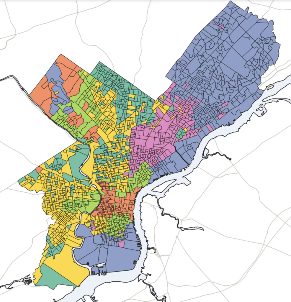
First, what wards are “Open”? As I said, there’s no single definition. But for this analysis, I’m using the set of Wards that have bylaws allowing committeepeople to vote on endorsements. Those I’m considering Open are:
| 1 |
2018 |
| 2 |
2018 |
| 5 |
60s or 70s |
| 8 |
60s or 70s |
| 9 |
60s or 70s |
| 15 |
2022 |
| 18 |
2018 |
| 24 |
2022 |
| 27 |
60s or 70s |
| 30 |
1998 |
| 39a |
2022 |
(If you want to contest these definitions or years, my email is
open.)
View code
library(sf)
library(dplyr)
library(tidyr)
library(ggplot2)
source("../../admin_scripts/theme_sixtysix.R")
source("../../admin_scripts/util.R")
asnum <- function(x) as.numeric(as.character(x))

divs <- st_read("../../data/gis/warddivs/202011/Political_Divisions.shp")ward_from_div <- function(warddiv){
  ward <- substr(warddiv, 1, 2)
  div <- substr(warddiv, 4,5)
  ward <- case_when(
    ward == "39" & asnum(div) >= 25 ~ "39a",
    ward == "39" & asnum(div) < 25 ~ "39b",
    TRUE ~ ward
  )
  return(ward)
}

divs <- divs |>
  mutate(
    warddiv = pretty_div(DIVISION_N),
    ward = ward_from_div(warddiv)
  )

wards <- divs |> group_by(ward) |> summarise() |> st_make_valid()

open_wards <- tribble(
  ~ward, ~year_opened,
  "01", "2018",
  "02", "2018",
  "05", "60s or 70s",
  "08", "60s or 70s",
  "09", "60s or 70s",
  "15", "2022",
  "18", "2018",
  "24", "2022",
  "27", "60s or 70s",
  "30", "1998",
  "39a", "2022"
)

wards <- wards |> mutate(
  is_open = ward %in% open_wards$ward,
  is_open_pre_22 = ward %in% (
    open_wards |> filter(year_opened != "2022") |> with(ward)
  )
)

ggplot(wards) +
  geom_sf(aes(fill = is_open)) +
  scale_fill_manual(
    values=c(`TRUE` = light_blue, `FALSE` = light_grey),
    guide=FALSE
  ) +
  geom_text(
    data = wards |> filter(is_open) |>
      mutate(
        x = st_coordinates(st_centroid(geometry))[,"X"],
        y = st_coordinates(st_centroid(geometry))[,"Y"]
      ),
    aes(
      x = x,
      y = y,
      label = ward
    ),
    size = 3
) +
  theme_map_sixtysix() +
  labs(
    title="Philadelphia's Open Wards"
  )

The first thing you’ll notice is that these wards cluster around
Center City. As such, they tend to be wealthier and whiter than the city
as a whole; the same demographics that have seen a generalized surge in turnout
since 2016. That makes the causality here difficult to measure: does
the openness of a ward increase turnout, or did these wards become open
thanks to local political engagement, and turnout there would have increased
regardless?
There’s another complication in answering the question: how should we
define turnout? I don’t love the usual measure, votes cast divided by
registered voters; that number will be alarmingly low because of inactive voters still on the rolls, and the denominator moves for all sorts of reasons,
including slow cleaning of the voter rolls or registration drives (I’ve
called this the Turnout
Funnel). And wards might have very different populations with
different propensities to vote, or even be eligible to vote, which we want to control for.
I’ll use my favorite metric: turnout in an off-year election as a
percentage of Presidential turnout. Off-year turnout is more malleable
to local GOTV efforts: there’s more need just to remind people when
Election Day is, and people get less communication about the election
from other channels. A division’s Presidential turnout gives a ceiling
on plausible off-year turnout. In this case, I’ll measure turnout in
November 2022 divided by turnout in November 2020.
View code
df_major <- readRDS("../../data/processed_data/df_major_20230116.Rds")

turnout <- df_major |> filter(is_topline_office, ward != "99") |>
  group_by(warddiv, year, election_type) |>
  summarise(votes=sum(votes))

turnout <- turnout |> left_join(
  divs |> as.data.frame() |> select(warddiv, ward),
  by="warddiv"
) |>
  left_join(
    wards |> as.data.frame() |> select(ward, is_open, is_open_pre_22),
    by="ward"
  )

div_turnout <- turnout |>
  pivot_wider(
    names_from=c("election_type", "year"),
    values_from = "votes"
  )

ward_turnout <- turnout |>
  group_by(ward, year, election_type, is_open, is_open_pre_22) |>
  summarise(votes=sum(votes)) |>
  pivot_wider(names_from=c("election_type", "year"), values_from="votes")

ward_turnout |>
  mutate(row = case_when(is_open ~ ward, TRUE ~ "Closed Wards")) |>
  group_by(is_open) |>
  summarise(votes_20 = sum(general_2020), votes_22 = sum(general_2022, na.rm=T)) |>
  mutate(ratio = votes_22 / votes_20)
View code
ggplot(wards |> left_join(ward_turnout, by="ward", suffix=c("", "_w"))) +
  geom_sf(aes(fill = general_2022 / general_2020)) +
  geom_sf(aes(color=is_open), fill = NA, lwd=1) +
  scale_color_manual(guide=FALSE, values=c(`TRUE` = "white", `FALSE` = alpha("white", 0))) +
  scale_fill_viridis_c() +
  theme_map_sixtysix() %+replace%
  theme(legend.position = "right") +
  labs(
    title="Turnout in 2022 vs 2020",
    subtitle="Open Wards are outlined.",
    fill = "Votes cast \n2022 / 2020"
  )

Overall, the Open Wards (including those that only became Open later)
cast 148,000 votes for President in 2020, and then 118,000 for Governor
in 2022, an 80% rate. The other wards cast 594,000 and 380,000, a 64%
rate. That’s a 16 percentage point difference!
But it might not be causal. We need to control for the ways Open
Wards are systematically difference from Closed ones. We could
do this by adding a bunch of control variables to a regression, but
I prefer a stronger approach: using spatial boundary discontinuities. We
can look at neighboring divisions on opposite sides of a ward boundary,
one in a closed ward and one in an Open Ward) and compare the
differences. By using only neighboring divisions, we create a useful
apples-to-apples comparison; we assume that any systematic differences
between these divisions is the effect of Open Wards. (I did a similar
analysis in 2019, measuring the
power of ward endorsements.)
For this analysis, I’ll limit to wards that were only Open before
2022 (sadly excluding my own 24). I filter down so each division is only
in a single pair, and control for the proportions Black and Hispanic in
the divisions (the pairing of divisions across boundaries should mean
these proportions are not that different, but this will control for any
lingering differences that do exist).
View code
block_data <- readr::read_csv(
  "../../data/census/decennial_2020_poprace_phila_blocks/DECENNIALPL2020.P4_data_with_overlays_2021-09-22T083940.csv",
  skip=1
)
block_shp <- sf::st_read(
  "../../data/gis/census/tl_2020_42101_tabblock/tl_2020_42_tabblock20.shp"
)block_shp <- st_transform(block_shp, st_crs(wards))
block_cents <- block_shp |> st_centroid()

st_contains_df <- function(shp1, shp2, id1, id2){
  raw <- st_contains(shp1, shp2)
  res <- list()
  for(i in 1:length(id1)){
    res[[i]] <- data.frame(
      id1 = id1[i],
      idx2 = raw[[i]],
      id2 = id2[raw[[i]]]
    )
  }
  return(bind_rows(res))
}

blocks_to_wards <- st_contains_df(wards, block_cents, wards$ward, block_cents$GEOID20) |>
  rename(ward = id1, block_i = idx2, geoid = id2)

res <- list()
for(ward in unique(blocks_to_wards$ward)){
  blocks_w <- block_cents[
    blocks_to_wards |> filter(ward == !!ward) |> with(block_i),
  ]
  divs_w <- divs |> filter(ward == !!ward)
  blocks_to_divs <- st_contains_df(divs_w, blocks_w, divs_w$warddiv, blocks_w$GEOID20) |>
    select(-idx2) |>
    rename(warddiv = id1,  geoid = id2)
  res[[ward]] <- blocks_to_divs
}
blocks_to_divs <- bind_rows(res)

div_pops <- blocks_to_divs |>
  inner_join(block_data |> mutate(geoid = substr(id, 10,24)), by="geoid") |>
  group_by(warddiv) |>
  summarise(
    pop = sum(`!!Total:`),
    hisp = sum(`!!Total:!!Hispanic or Latino`),
    nhw =  sum(`!!Total:!!Not Hispanic or Latino:!!Population of one race:!!White alone`),
	nhb = sum(`!!Total:!!Not Hispanic or Latino:!!Population of one race:!!Black or African American alone`),
    nha = sum(`!!Total:!!Not Hispanic or Latino:!!Population of one race:!!Asian alone`)
  )
neighboring_wards <- st_touches(wards)
neighboring_wards <- neighboring_wards |>
  lapply(as.data.frame) |>
  bind_rows(.id = "id0") |>
  mutate(id0 = asnum(id0)) |>
  rename(id1 = `X[[i]]`) |>
  filter(id0 < id1) |>
  mutate(ward0 = wards$ward[id0], ward1 = wards$ward[id1])

neighboring_divs <- vector(mode="list", length=nrow(neighboring_wards))
for(row in 1:nrow(neighboring_wards)){
  ward0 <- neighboring_wards$ward0[row]
  ward1 <- neighboring_wards$ward1[row]

  divs0 <- divs |> filter(ward == ward0)
  divs1 <- divs |> filter(ward == ward1)
  touches <- st_touches(divs0, divs1) |>
    lapply(as.data.frame) |>
    bind_rows(.id = "id0") |>
    mutate(id0 = asnum(id0)) |>
    rename(id1 = `X[[i]]`) |>
    mutate(div0 = divs0$warddiv[id0], div1 = divs1$warddiv[id1])
  neighboring_divs[[row]] <- touches |> select(div0, div1)
}
neighboring_divs <- bind_rows(neighboring_divs)

neighboring_divs <- neighboring_divs |>
  left_join(
    div_turnout, by=c("div0"="warddiv")
  ) |>
  left_join(
    div_turnout, by=c("div1"="warddiv"),
    suffix=c("_0", "_1")
  ) |>
  left_join(
    div_pops, by=c("div0" = "warddiv")
  )|>
  left_join(
    div_pops, by=c("div1" = "warddiv"),
    suffix=c("_0", "_1")
  )

neighboring_divs <- neighboring_divs |>
  mutate(
    prop_22_over_20_0 = general_2022_0 / general_2020_0,
    prop_22_over_20_1 = general_2022_1 / general_2020_1,
    signed_is_open = is_open_1 - is_open_0,
    signed_is_open_pre_22 = is_open_pre_22_1 - is_open_pre_22_0
  )

# Grab arbitrary unique pairs
set.seed(215)
neighboring_divs_lm <- neighboring_divs |>
  group_by(div0) |>
  filter(sample.int(n()) == 1) |>
  group_by(div1) |>
  filter(sample.int(n()) == 1)

form <- as.formula(
  "prop_22_over_20_1 - prop_22_over_20_0 ~ -1 + signed_is_open_pre_22 + I(hisp_1 / pop_1 - hisp_0 / pop_0) + I(nhb_1 / pop_1 - nhb_0 / pop_0)"
)
fit <- lm(form, data = neighboring_divs_lm)
summary(fit)
##
## Call:
## lm(formula = form, data = neighboring_divs_lm)
##
## Residuals:
##      Min       1Q   Median       3Q      Max
## -0.31756 -0.05978 -0.00070  0.04634  0.32425
##
## Coefficients:
##                                Estimate Std. Error t value Pr(>|t|)
## signed_is_open_pre_22           0.01738    0.01503   1.156    0.248
## I(hisp_1/pop_1 - hisp_0/pop_0) -0.26663    0.06638  -4.017 7.38e-05 ***
## I(nhb_1/pop_1 - nhb_0/pop_0)   -0.24061    0.03274  -7.349 1.72e-12 ***
## ---
## Signif. codes:  0 '***' 0.001 '**' 0.01 '*' 0.05 '.' 0.1 ' ' 1
##
## Residual standard error: 0.09265 on 316 degrees of freedom
## Multiple R-squared:  0.1924, Adjusted R-squared:  0.1847
## F-statistic:  25.1 on 3 and 316 DF,  p-value: 1.37e-14
The result: divisions in Open Wards had 1.7pp stronger turnout than
divisions just across the boundary, but this result has a p-value of
0.25 and is not statistically significant (meaning we don’t have enough
data to be confident it’s different from zero). This provides a
confidence interval of (-1pp, 5pp).
A few notes about this analysis:
- The result was much bigger (about 5pp) when I didn’t control for
race! This means that even when comparing only division across
boundaries, there are racial differences between the divisions in Open
Wards and those not.
- I’m only using one election comparison (2022 vs 2020), and we
obviously have a lot more. I’ll think about ways to compellingly use
more elections without introducing complications. Quick checks using
2018 vs 2016 did not substantively change the results.
So, what does this mean? Our best estimate for Open Wards’ change in
turnout is a small, positive effect, but we don’t have enough data to be
confident this is different from zero. Open Wards of course have other
claims to benefits than just turnout: more democratic decision-making,
for example. And a 2 percentage point increase in Philadelphia’s
turnout, if it existed, wouldn’t be nothing: if scaled across the city,
it would have meant 4,000 votes in 2019’s Superior Court election, which
was decided by 17,000.