Recent push-back has argued that simply nobody changes their minds anymore, and the people who do probably aren’t all that likely to vote anyway. What really matters is energizing your base, and making sure they vote. There can be once-a-generation political realignments, but for the most part people just vote for their party. The difference between victories for one party or another is which party is more energized.
There are smarter people than me having this debate (my favorite recent book has been the eye-opening Democracy for Realists), but what I can do is look at the Philadelphia version. Where in Philadelphia does Turnout matter? Where does Persuasion?[1]
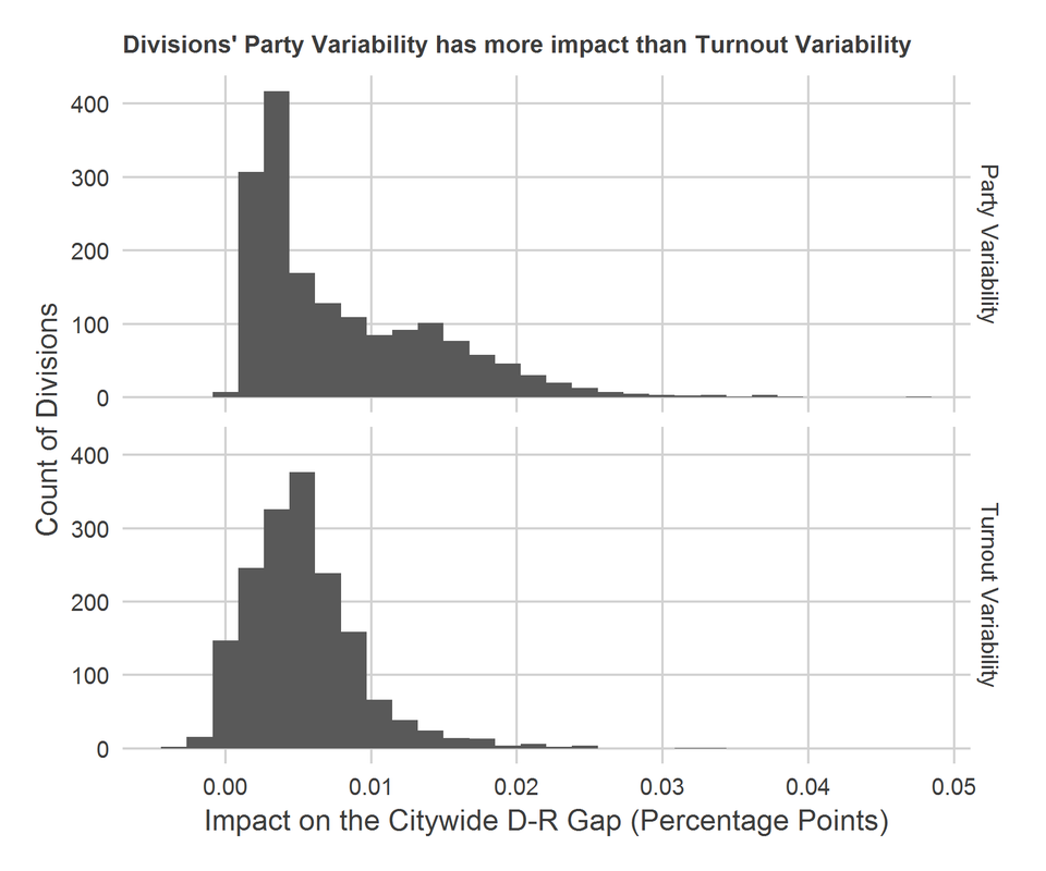
One of the favorite tools of demographers is the decomposition. This is a (surprisingly simple) mathematical technique for breaking down the change in something into the relative importance of the change in its constituent parts. In the footnotes, I develop a formula that decomposes a the variability in a party’s win total (measured as the gap in votes between the winning party and the losing party) into variability of turnout plus variability of party preference. The equation boils down to
Variability in Gap = (Variability in Preferences) x (Average Turnout) + (Variability in Turnout) x (Average Preference)
= (Party Variability Component) + (Turnout Variability Component)
The equation reveals two campaign strategies, by maximizing each of the two addends:
(1) maximize the first component by persuading voters in divisions with variable preferences and high turnout.
(2) maximize the second component by turning out voters in divisions with highly variable turnout, where the average preference is strongly for your party.
These components boil down to obvious strategies, but the decomposition gives us a way to score divisions based on each. A division’s score along each component tells us what impact that division has changes in the citywide election.
Party variability measures the impact on the citywide Democrat-Republican gap that a division’s preference swings have. A division with a score of 0.02 means that when a division changes its party percentage by its average swing, the citywide vote total changes by 0.02 percentage points. This will depend on (1) how swing-y that division is, i.e. what constitutes its “average swing”, and (2) its typical turnout. Divisions that swing between Democrats and Republicans, and where everyone votes, will have high scores.
Turnout variability measures the impact on the gap that a division’s turnout swings have. A division with a score of 0.02 means that when a division increases its turnout by its average swing, the citywide vote total changes by 0.02 percentage points. This will depend on (1) how much turnout varies in that district, which determines its “average swing”, and (2) its typical party gap. Divisions where turnout varies wildly but which is strongly Democratic or Republican will have high scores.
(I use “relative turnout”, which is a division’s proportion of the citywide total, rather than vote counts. Thus, large swings for a Presidential election aren’t considered a swing unless the division votes disproportionately more than other divisions in that year. This also means that citywide turnout efforts won’t affect the score, only localized ones.)
I expect this result to reverse when we zoom out to the state level; relative turnout variability is likely much higher between the city and the rest of the state than it is within the city.
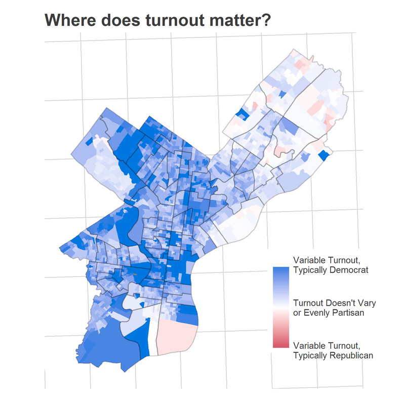
Turnout will matter in divisions where the percentage of voters varies from year to year, and where voter preferences are overwhelmingly Democratic or Republican. The map below colors divisions by the turnout component score, with the hue representing whether Republicans or Democrats benefit from an increase in turnout. The Northeast and Manayunk have low scores–they are too split between parties for turnout to help one party more than another. West Philly also has surprisingly low scores: turnout there is simply too stable for turnout efforts to have an effect (except for in University City). Interestingly, the predominately-Hispanic section of North Philly has very high scores: voters turn out for Presidential elections and not for other elections, and they vote overwhelmingly Democratic.
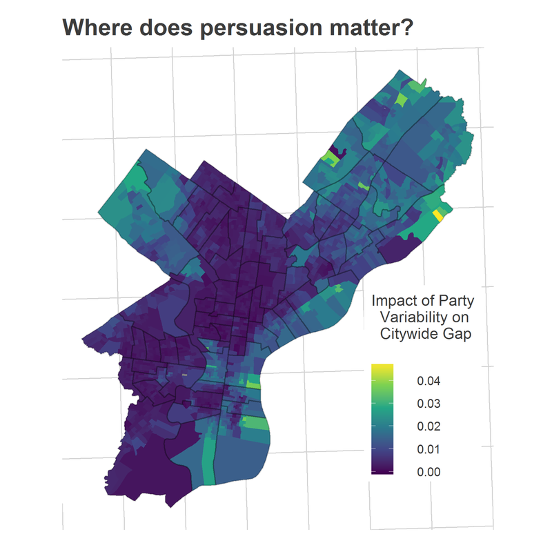
Persuasion campaigns will have an impact in divisions where the party preferences vary from election to election, and where turnout is always high. The map below colors divisions by their party preference score. The Northeast, Manayunk, and Port Richmond now light up: these are all neighborhoods where people vote at high rates, and swing between Democrats and Republicans. North Philly and West Philly are simply too consistent in party preferences–Democrats win with 99% of the vote–for convincing to matter.
Our most important upcoming election is the 2018 race for Governor. In a future post, I will replicate this analysis at the state level. What counties can be persuaded? What counties need to be mobilized? I expect that the state results could be very different than for within Philadelphia. Stay tuned!
[1] Of course, strategies for convincing and strategies for turnout are not so separable. There are probably a lot of campaign actions that achieve both.
First, I’ll motivate demographers’ common decomposition in the case of only two years, then I’ll expand it to a multi-year version. (Apologies for the hideous math, I haven’t been able to figure out how to typeset math in this blog yet.)
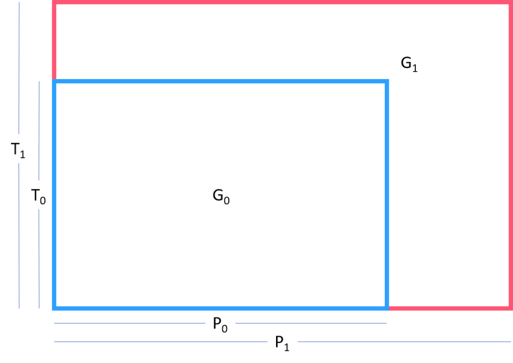
Suppose we have a value G that is the product of two numbers, P and T. In the current case, G is the citywide vote gap between Democrats and Republicans, defined as the total votes for Democrats minus the total votes for Republicans. P is the percentage gap between Democrats and Republicans, and T is the total turnout in votes. Notice that
G = P * T
Consider the case where we observe these values in two time periods, 0 and 1. We are interested in what caused the gap G to change between year 0 and year 1. It could be changes in the percentage P (call this persuasion) or changes in turnout T (call this mobilization). That is, we are interested in G_1 – G_0. We can write
G_1 – G_0 = (P_1 * T_1) – (P_0 * T_0)
A little bit of algebra can show that:
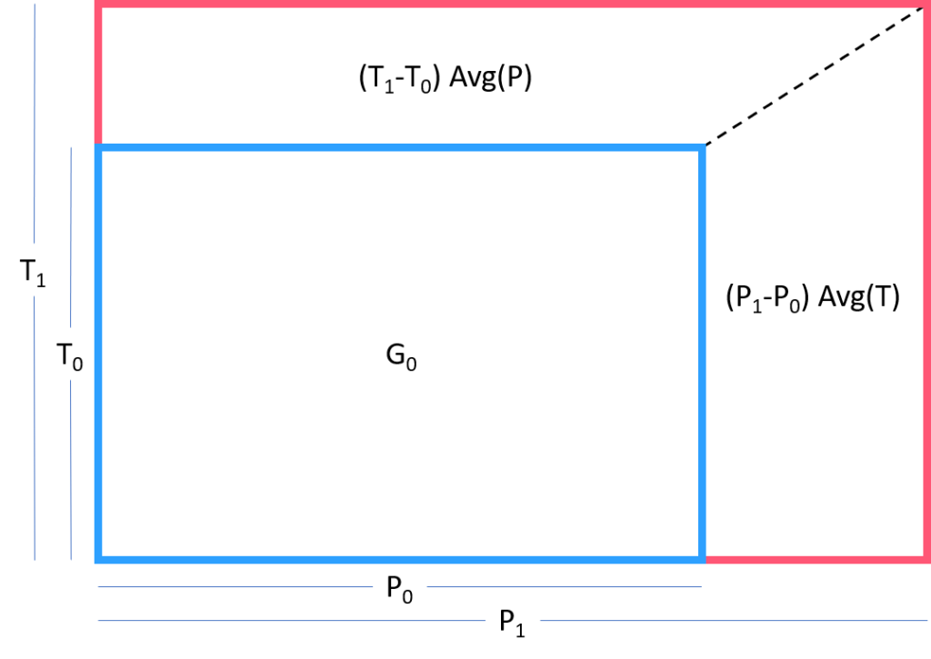
G_1 – G_0 = (P_1 – P_0) * Avg(T) + (T_1 – T_0) * Avg(P)
These two addends are our components. The first addend can be interpreted as the change in the vote gap due to the changes in the proportion voting for the Democrat, scaled by the average number of voters. The second is the change in the gap due to changes in the total people voting, scaled by the average party preference.
A simple picture helps build intuition for this decomposition. Below, we are interested in the difference of the areas of the two rectangles, G_1 and G_0. Notice that the area of each can be written as base times height, or P * T. The area from G_0 to G_1 changes both because P changes and T changes. But how much of the change was due to P, and how much due to T?
We aren’t limited to doing this for only the city as a whole. We can calculate this decomposition for each division. The total gap in the city is the sum of the gaps in each precinct. The total state gap is given by summing over each precinct i:
G_1 – G_0 = SUM(G_i1 – G_i0)
= SUM(P_i1 * T_i1 – P_i0 * T _i0)
= SUM( (P_i1 – P_i0) * Avg(T_i) + (T_i1 – T_i0) * Avg(P_i) )
= SUM( Preference_Component_i + Turnout_Component_i)
We can thus calculate each precinct’s two scores, and then the total change in the city-wide gap between year 0 and year 1 as the sum of both scores for all precincts.
Thus far we’ve only been using two years. However, we want to be able to incorporate all of the elections at once.
The absolute value of the first term can be written as
|(P_i1 – P_i0) * Avg(T_i)| = (|(P_i1 – Avg(P_i)| + |(P_i0 – Avg(P_i)|) * Avg(T_i),
(this relies on the fact that Avg(P_i) is between P_i0 and P_i1). This may look complicated, but it has a nice interpretation: it is the size of typical deviation of P_i from its average value, scaled by the average turnout.
We similarly write
|(T_i1 – T_i0)| * Avg(P_i) = (|(T_i1 – Avg(T_i)| + |(T_i0 – Avg(T_i)|) * Avg(P_i)
Where I’ve left P_i outside of the absolute value so the sign captures partisanship: positive values represent a Democratic gap, negative a Republican gap (signs are arbitrary).
This inspires a multi-year version of the decomposition:
Decomposed Variability = Avg(|P_ij – Avg(P_i)|) * Avg(T_i) + Avg(|T_ij – Avg(T_i)|) * Avg(P_i)
= Preference Variability Component + Turnout Variability Component
Notice that the last term does not use the absolute value on P_i. This means that it will have the sign of the typical partisan gap, and thus the last term is capable of showing which party an increase in turnout will help.
(Statsy readers: Avg(|P_ij – Avg(P_i)|) is like a linear version of the variance).
This allows us to score a county i based on whether its percent-Democrat varies more, or its turnout. It’s no longer an accounting identity, but it does simplify to the accounting identity above when you only consider two years.
We could be done here, but to really compare across years, I divide a precinct’s vote total by that year’s City vote total, T_j. This means that the left hand side can be interpreted as the percentage gap between Democrats and Republicans, rather than a raw vote count. For example, if the Republican won 52% to 48%, the gap would be 4 percentage points.
Decomposed Pct Gap = Avg(|P_ij – Avg(P_i)|) * Avg(T_ij / T_j) + Avg(|T_ij/T_j – Avg(T_ij/T_j)|) * Avg(P_i)